How much hardware does your on-premise LLM need?

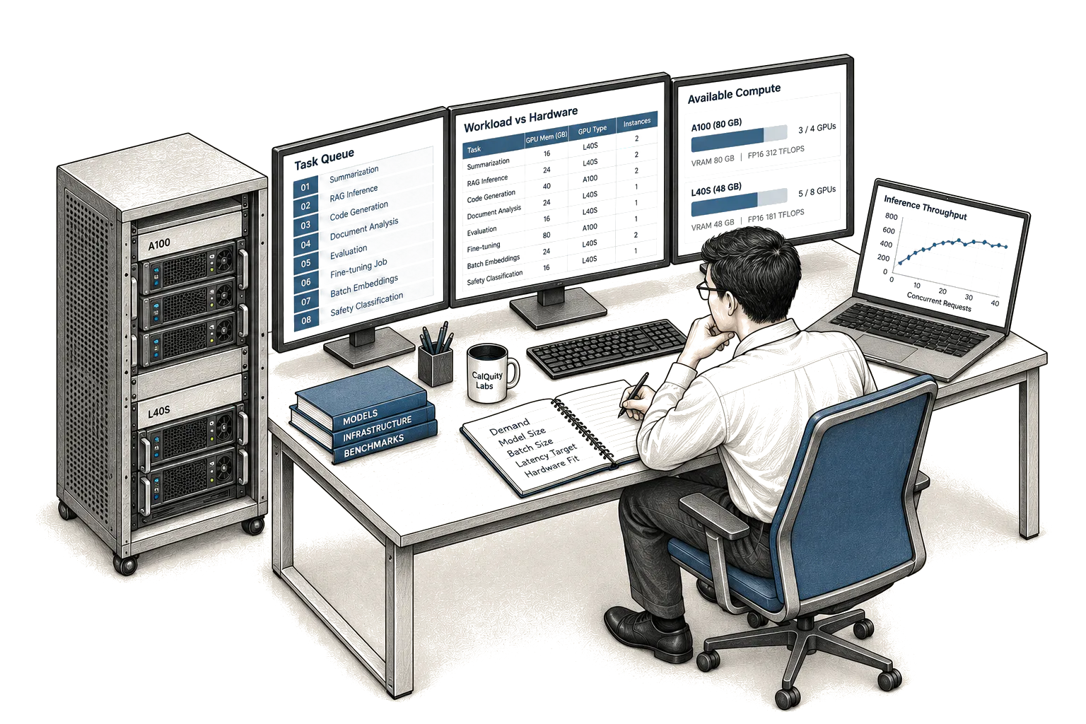
Size the request queue before choosing the GPU

An on-premise LLM needs enough hardware to serve the peak concurrent request set inside its latency deadline. Parameter count establishes the weight footprint, but concurrency, context length, and latency determine whether the deployment needs one accelerator or several.

Consider Llama 3.3 70B Instruct. Its BF16 weights occupy 141,107,557,487 bytes, about 141.1 GB or 131.4 GiB, before the server allocates any key-value cache ¹. That fact rules out an 80 GB H100 for BF16 weights. It does not tell you whether the deployment needs two H200s, three H100s, or a larger replicated pool.

The missing inputs are operational:

• How many requests will be generating tokens simultaneously?
• How many input and output tokens must each request retain?
• What time to first token and inter-token latency must the service meet?
• How much traffic arrives in bursts rather than at the average rate?
• Which model precision passes the application's quality tests?

"Concurrent users" is not yet a sizing input. A workforce with 200 logged-in users and an assumed active fraction of 10 percent creates a modelled concurrency of 20 requests only if each active user has one request in flight. An agent that launches four parallel model-generation calls changes the same estimate to 80 in-flight model requests. Tool or retrieval calls count toward GPU concurrency only when they invoke the model. Both figures are estimates derived from the stated assumptions, not measurements.

Picture a platform engineer scoping hardware for a claims-processing assistant against exactly that roster: 200 named users, 10 percent assumed active, 20 concurrent requests written into the procurement memo as the sizing basis. The application later ships as an agent that fans each user turn into several parallel model-generation calls, and the same roster now produces the 80-request estimate two paragraphs above it, a figure the memo never revisited because the user count on the roster never changed.

This distinction also affects application design. A chatbot, copilot, and workflow agent create different arrival patterns even when the user count is identical. The choice should be settled before procurement, as described in Chatbot, copilot, workflow, or AI agent?.

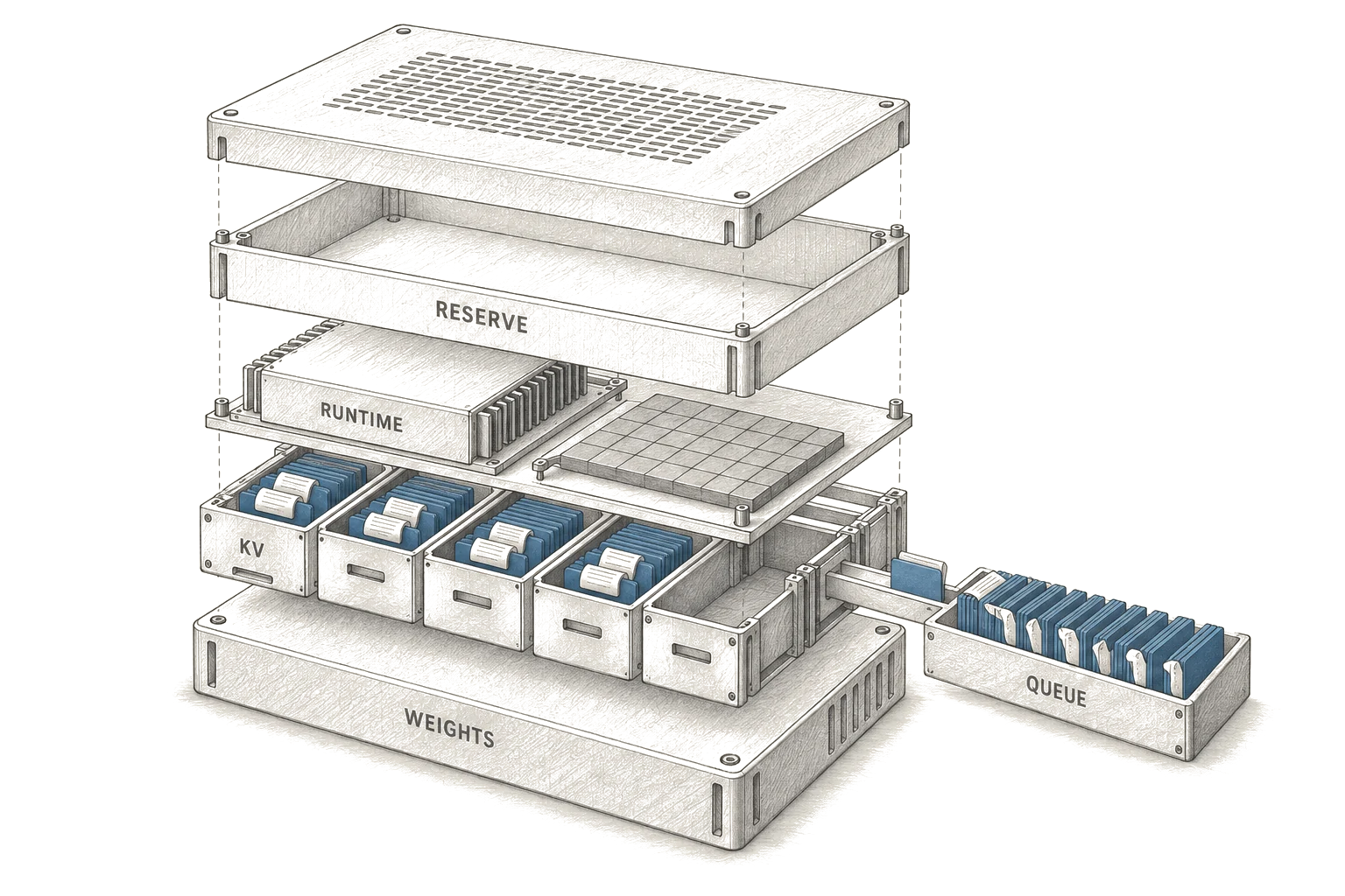
GPU memory must hold weights, KV cache, and operating reserve

The capacity calculation is:

working set =
    model weights
  + KV cache for all active sequences
  + serving runtime allocations
  + temporary execution workspace
  + operating reserve

Weights are mostly fixed after selecting the model and precision. The KV cache is workload-dependent. NVIDIA states that its memory footprint grows linearly with batch size and sequence length ². Doubling active sequences therefore doubles the KV allocation if their cached lengths remain equal. Doubling context length has the same effect.

The correct KV coefficient is model-specific. It depends on layer count, attention dimensions, KV head count, cache precision, tensor-parallel layout, and serving implementation. Obtain it from the exact model and runtime configuration rather than copying a generic bytes-per-token value.

The coefficient then turns capacity planning into straightforward arithmetic:

KV bytes =
    active sequences
  × cached tokens per sequence
  × measured KV bytes per token

Sequence lengths vary, so multiplying the maximum context by the maximum batch is a conservative bound rather than a forecast. A better workload model uses the observed distribution of cached tokens at peak traffic, then reserves explicit capacity for the tail.

Memory management changes the usable fraction. The vLLM project reports that serving systems before paged KV memory management wasted 60 to 80 percent of memory through fragmentation and over-reservation ³. PagedAttention reduces that waste. It does not make KV memory independent of concurrency or context.

In vLLM, max_num_seqs and max_num_batched_tokens expose this trade directly. Lowering either setting reduces concurrent work and frees KV cache space ⁴. An out-of-memory error can therefore be removed by reducing concurrency, but the requests move into the scheduler queue. Capacity improves while queueing latency worsens.

Decode is usually bandwidth-bound, while long prefills move the bottleneck

Autoregressive decode repeatedly reads model weights to produce the next token. NVIDIA describes model execution as frequently bandwidth-bound in the weights ². This is why two accelerators with enough combined memory can deliver different latency even when both hold the same model.

The relevant specifications show the spread. An H100 configuration provides 80 GB at 3.35 TB/s, while another H100 configuration provides 94 GB at 3.9 TB/s ⁵. An H200 provides 141 GB at 4.8 TB/s ⁶. An L40S provides 48 GB at 864 GB/s ⁷.

Capacity and bandwidth must be tested separately. Five L40S accelerators provide a modelled 240 GB of aggregate memory and 4.32 TB/s of aggregate bandwidth, derived by multiplying the published per-card specifications by five and assuming perfect distribution. Two H200s provide a modelled 282 GB and 9.6 TB/s under the same ideal assumption. Neither calculation includes communication overhead, topology limits, runtime overhead, or idle capacity caused by uneven sharding.

A bandwidth ceiling can be estimated before benchmarking. Dividing the H200's published 4.8 TB/s by the model's 141.1 GB BF16 weight footprint gives a modelled upper bound of about 34 complete weight reads per second on one card. Two H200s under ideal tensor-parallel scaling raise that estimate to about 68 reads per second. This is a screening calculation, not measured token throughput.

Prefill behaves differently. Processing a prompt is a parallel matrix-matrix operation that can saturate GPU compute ². A deployment with long retrieved documents can therefore miss its time-to-first-token target even when decode bandwidth appears sufficient.

Chunked prefill addresses the scheduling interaction by mixing compute-bound prefill work with memory-bound decode work. vLLM documents the feature as improving throughput and latency by balancing those phases ⁴. The result still depends on prompt lengths and scheduler settings, so the actual workload must be benchmarked.

A worked estimate turns concurrency into accelerator count

The following model demonstrates the sizing process. It has not been measured on production hardware.

Assume Llama 3.3 70B Instruct at BF16, 16 simultaneously active sequences, 8,192 cached tokens per sequence, and an assumed KV allocation of 0.5 MiB per cached token. Also assume an operating reserve equal to 10 percent of weights plus KV cache. The KV coefficient and reserve are planning assumptions that must be replaced with profiler output from the intended serving stack.

The modelled KV allocation is:

16 × 8,192 × 0.5 MiB
= 65,536 MiB
= 64 GiB
= about 68.7 GB

Adding the sourced 141.1 GB weight footprint produces a modelled 209.8 GB subtotal. Applying the assumed 10 percent reserve produces a modelled working set of about 230.8 GB.

Capacity alone therefore requires two 141 GB H200s, providing a modelled 282 GB total, or three 80 GB H100s, providing a modelled 240 GB total. Two 80 GB H100s can hold the weights but cannot hold this modelled working set.

Latency supplies the second gate. Assume each request must generate 512 output tokens within 30 seconds after spending 2 seconds on queueing and prefill. The decode phase then has 28 seconds, so each active sequence requires a modelled average of about 18.3 output tokens per second, derived from 512 divided by 28. A production benchmark must show that all 16 sequences meet this rate at the selected tail-latency target.

The accelerator count is the larger result from two tests:

capacity count =
    working-set bytes
    divided by usable bytes per accelerator,
    rounded up

service count =
    required aggregate request rate
    divided by measured rate per replica at the latency target,
    rounded up

If capacity says two cards and the service benchmark says four, the deployment needs four. Buying two because the model fits produces a queueing problem rather than a memory problem.

A hardware buyer who signs off on two 80 GB H100s because the vendor's spec sheet confirms the weights fit is closing the capacity test and skipping the service test. The cards boot the model without incident. The queue that backs up past the latency deadline once real traffic arrives is not a hardware failure; it is the sizing step the purchase order never asked for.

The purchase price follows the configuration, not the model name

A cost teardown should preserve vendor quote lines as variables until procurement supplies them:

acquisition cost =
    accelerator quantity × quoted accelerator line price
  + host chassis
  + memory and storage
  + network fabric
  + support
  + installation

Operating cost should be calculated separately:

operating cost =
    measured average system kW
  × operating hours
  × facility electricity tariff
  × facility overhead factor

An illustrative procurement estimate shows why card count matters. Assume an H200 accelerator line price of $35,000, an H100 accelerator line price of $25,000, a two-accelerator host allocation of $20,000, a three-accelerator host allocation of $25,000, and $10,000 for storage and network equipment in either configuration. These are explicit modelling assumptions, not current market prices or vendor quotes.

Under those assumptions, the two-H200 configuration has a modelled acquisition cost of $100,000: two times $35,000, plus $20,000, plus $10,000. The three-H100 configuration has a modelled acquisition cost of $110,000: three times $25,000, plus $25,000, plus $10,000. Support, installation, tax, redundancy, and operating cost are excluded from both estimates.

The example does not establish that H200 is generally cheaper. It shows that a higher unit price can produce a lower system estimate when additional cards and a larger host are required. Replace every assumed price with a written quote and keep the arithmetic visible.

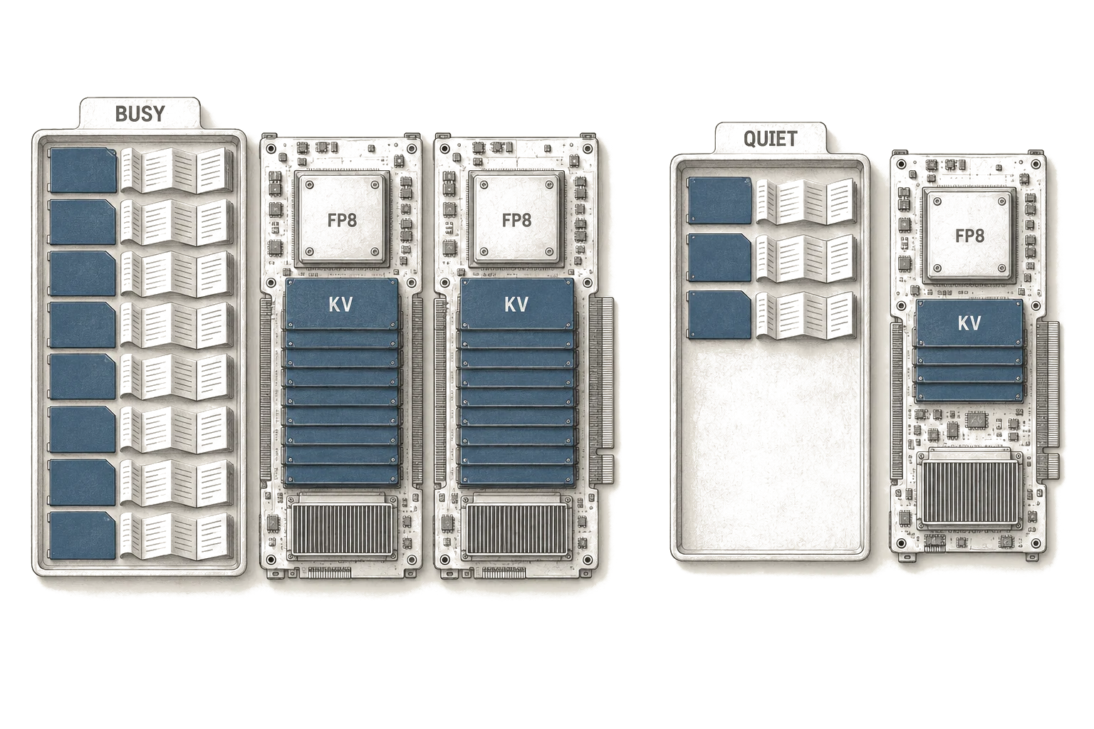
Quantization changes the answer only after concurrency is included

FP8 quantization can halve model memory requirements and improve throughput by up to 1.6 times, with the vLLM documentation reporting minimal accuracy impact ⁸. "Up to" is not a service-level guarantee, and application quality still requires evaluation on representative inputs.

Applying the documented twofold memory reduction to the 141.1 GB BF16 weights gives a modelled FP8 weight footprint of about 70.6 GB. Keeping the worked example's 68.7 GB KV allocation and assumed 10 percent reserve produces a modelled working set of about 153.2 GB. That still exceeds one H200's published 141 GB capacity.

Reduce the assumed concurrency from 16 active sequences to 8, and the modelled KV allocation falls from 68.7 GB to about 34.4 GB. The resulting modelled working set is about 115.5 GB after the same reserve, which fits within one H200.

Neither the parameter count nor the quantization scheme changed between those two cases. What moved the deployment from needing two H200s to fitting on one was the concurrency assumption, the number a procurement conversation is least likely to revisit once quantization has already been credited with the savings.

A smaller model follows the same process. Its lower weight footprint creates more room for KV cache and reduces bytes read during decode, but the quality decision belongs to the application evaluation. The human review burden can also alter total operating cost, which is addressed in How much of my team's time will checking the AI take?.

Apply the model with a benchmark that preserves latency

1. Define the service target in request terms. Record peak arrivals, active sequences, input-token distribution, output-token distribution, time to first token, inter-token latency, and completion deadline. Separate interactive traffic from offline jobs.

2. Freeze the candidate configuration. Record the exact model revision, weight precision, cache precision, serving runtime version, tensor-parallel degree, scheduler limits, and accelerator variant. An "H100 test" is ambiguous until its memory capacity and form factor are named.

3. Measure the working set. Start the server with the intended context and concurrency limits. Capture weight allocation, KV capacity, temporary allocations, and the point where requests begin queueing or fail. Replace the assumed KV coefficient in the worksheet with the observed value.

4. Sweep offered concurrency while replaying representative prompt and output lengths. A throughput result counts only while the latency target holds. Dynamic batching deliberately trades latency for throughput, as Triton's batcher documentation states ⁹.

5. Price the smallest configuration that passes both the memory and latency gates. Then add the replication required for maintenance and failure tolerance. Apply quote prices to the complete server configuration rather than multiplying a headline accelerator price.

This model breaks when the workload definition is false

Averages conceal the failure cases. A mean context length cannot size KV cache when retrieved-document requests occasionally fill the context window. A mean arrival rate cannot size an interactive service with synchronized morning traffic. Model each important traffic class separately and combine them at the scheduler.

An operations lead who sized the assistant off its average weekday load discovers the gap on the morning every shift supervisor opens the handover tool within the same few minutes. The average arrival rate never predicted that cluster, because it was never a property of any single request; it was a property of how the shift schedule works.

Agents make "users" especially unreliable. One user action can create parallel planning, retrieval, tool, and verification calls. Retries can amplify the request count during downstream failures. The sizing input must come from in-flight model requests, not authenticated sessions.

Prefix caching and repeated system prompts can reduce prefill work, while speculative decoding can change throughput. CPU or storage offload can reduce accelerator memory pressure. Each technique changes the benchmark conditions, and offload introduces another data path whose latency must be included. None permits sizing from parameter count alone.

Hardware placement also does not settle privacy or authorization. Retrieved context changes prompt length, while its access rules must remain correct through retrieval and generation. How to preserve RAG access controls end to end covers that control path. Likewise, an on-premise location does not establish the system's privacy boundary; What makes an LLM private? identifies the other data flows that require review.

Finally, the worksheet cannot replace a saturation test on the exact server topology. Published memory and bandwidth establish feasibility bounds. Scheduler behavior, communication overhead, prompt shape, kernels, and application deadlines determine the deployable concurrency. If those conditions change, the accelerator count and cost estimate must be recalculated.